The uniqueness of SHAP depends on how you handle external information

Summary

SHapley Values for Additive exPlanations (SHAP; Lundberg & Lee, 2017) is a popular method for explaining black box model predictions. Lundberg & Lee (hereafter, L&L) consider the case where model inputs can be measured sequentially, and where the prediction can be updated as more and more information is acquired. In this setting, the update caused by incorporating a new piece of information depends on the existing information that has already been accounted for. That is, the update caused by adding a particular input feature depends on the order in which the inputs are measured. L&L suggest that the overall contribution of each feature be summarized by averaging that feature's marginal contribution across all possible input orderings. Roughly speaking, this has the effect of smoothing away the dependency on ordering.

The authors claim that this averaging approach is the only method that satisfies a certain list of intuitive conditions defined by the Shapley values from game theory (L&L Theorem 1). Notably absent from their list however is the well-known "Symmetry" condition, which requires that any two features that produce the same prediction updates be given the same explanation. This condition would effectively prevent the model explanation from being influenced by prior or external knowledge about either the problem domain or the way in which inputs tend to be measured. L&L state that Symmetry is not required to ensure a unique model explanation.

The primary goal of this comment is to point out that this last claim is in error. L&L implicitly assume that feature names don't matter in their proof, but feature names do matter if we incorporate prior knowledge into the explanation process. Modifying the theorem by explicitly adding a Symmetry requirement does ensure a unique solution, and such an addition may be reasonable in generic scenarios lacking prior knowledge. However, without the Symmetry constraint, any weighted combination over the set of possible orderings produces a valid solution. Indeed, applying weights to the different measurement orderings may be a useful way to incorporate prior knowledge.

For example, suppose two pieces of information are collected as part of a procedure to diagnose arm fractures: a physical exam for pain and swelling, and an x-ray. As the doctor collects each piece of information, they update their predicted probability of fracture. However, the extent to which physical exam results update the doctors prediction depends highly on whether or not an x-ray has already been performed. If the physical exam is done first, the results could dramatically influence the doctor's predicted probability of fracture. However, if the x-ray is done first, the subsequent physical exam might not make any marginal impact on the doctor's prediction. Indeed, partly for this reason, physical exams are almost always administered before x-rays. However, the prevalence of different measurement orderings does not factor into the SHAP computation. Instead, SHAP determines the influence of the physical exam by averaging (1) the marginal influence of the exam if the exam is done first, and (2) the marginal influence of the exam if the x-ray is done first. By placing equal weight on these two measurement orderings, SHAP can underestimate the value that physical exams tend to provide in practice.

In the next section I'll introduce the SHAP procedure with a slightly more complex example of COVID-19 screening based on three hypothetical risk factors. I'll then introduce more detailed notation in order to discuss L&L Theorem 1.

Note: I reached out to the SHAP paper's authors and had several helpful discussions while writing this comment.

Introducing SHAP with a hypothetical example of predicting COVID-19 status

To introduce the basic idea of SHAP, I'll consider a hypothetical example of predicting COVID-19 status among health-care workers. Suppose that an analyst observes a health-care worker with the following three characteristics:

1. no dry cough,
2. fever present, and
3. positive result on nasal swab test.

After seeing this information, the analyst assigns the health-care worker a 0.98 probability being infected.

SHAP decomposes the 0.98 predicted probability into components associated with each of these three pieces of evidence (A, B & C). I'll describe the SHAP procedure in more detail below. But, at a high level, in order to implement SHAP we'll need to know the risk prediction that the analyst would have made if only a subset of the above facts had been available. For example, suppose that¹

• when told no information, the analyst predicts a baseline probability of 0.10;
• when told only (A), the analyst predicts a 0.05 probability;
• when told only (B), the analyst predicts a 0.20 probability;
• when told only (C), the analyst predicts a 0.96 probability;
• when told only (A) & (B), the analyst predicts a 0.15 probability;
• when told only (A) & (C), the analyst predicts a 0.93 probability;
• when told only (B) & (C), the analyst predicts a 0.99 probability; and
• when told all three facts, the analyst predicts a 0.98 probability.

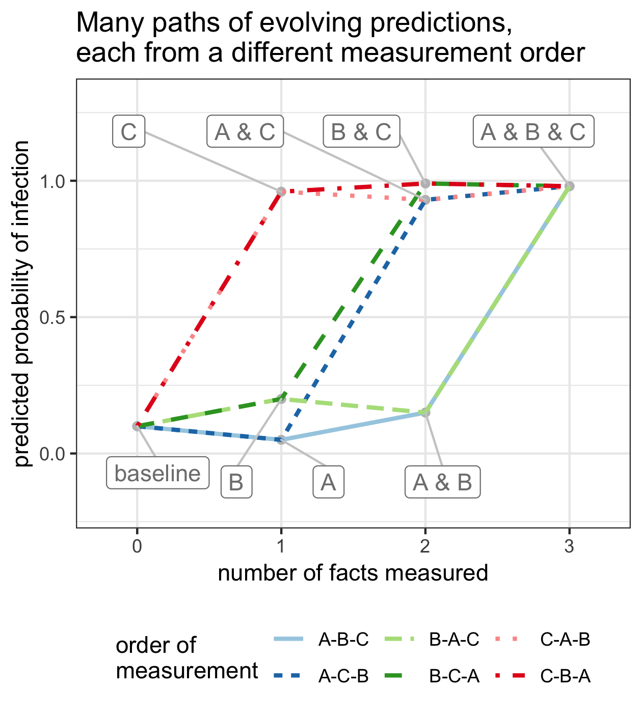
We can imagine that the analyst might learn facts (A), (B), and (C) in any of 6 possible orders: A-B-C, A-C-B, B-A-C, B-C-A, C-A-B, or C-B-A. For each order, we can consider how the analyst's risk prediction evolves as they learn more. For example, under the ordering B-C-A, the analyst's prediction moves from 10% (baseline) to 20% (B), then to 99% (B & C), and then to 98% (A & B & C). All six possible trajectories are shown below.

For each trajectory, we can also compute the change in predictions when each piece of information is added. For example, again considering the B-C-A ordering, the marginal contribution of fever (B) is \(0.20 - 0.10 = 0.10\); the marginal contribution of the positive nasal swab (C) is \(0.99 - 0.20 = 0.79\); and the marginal contribution of no cough (A) is \(0.98 - 0.99 = -.01\). Below, we show the marginal change in predictions associated with adding each of the three pieces of information, as a function of measurement order.

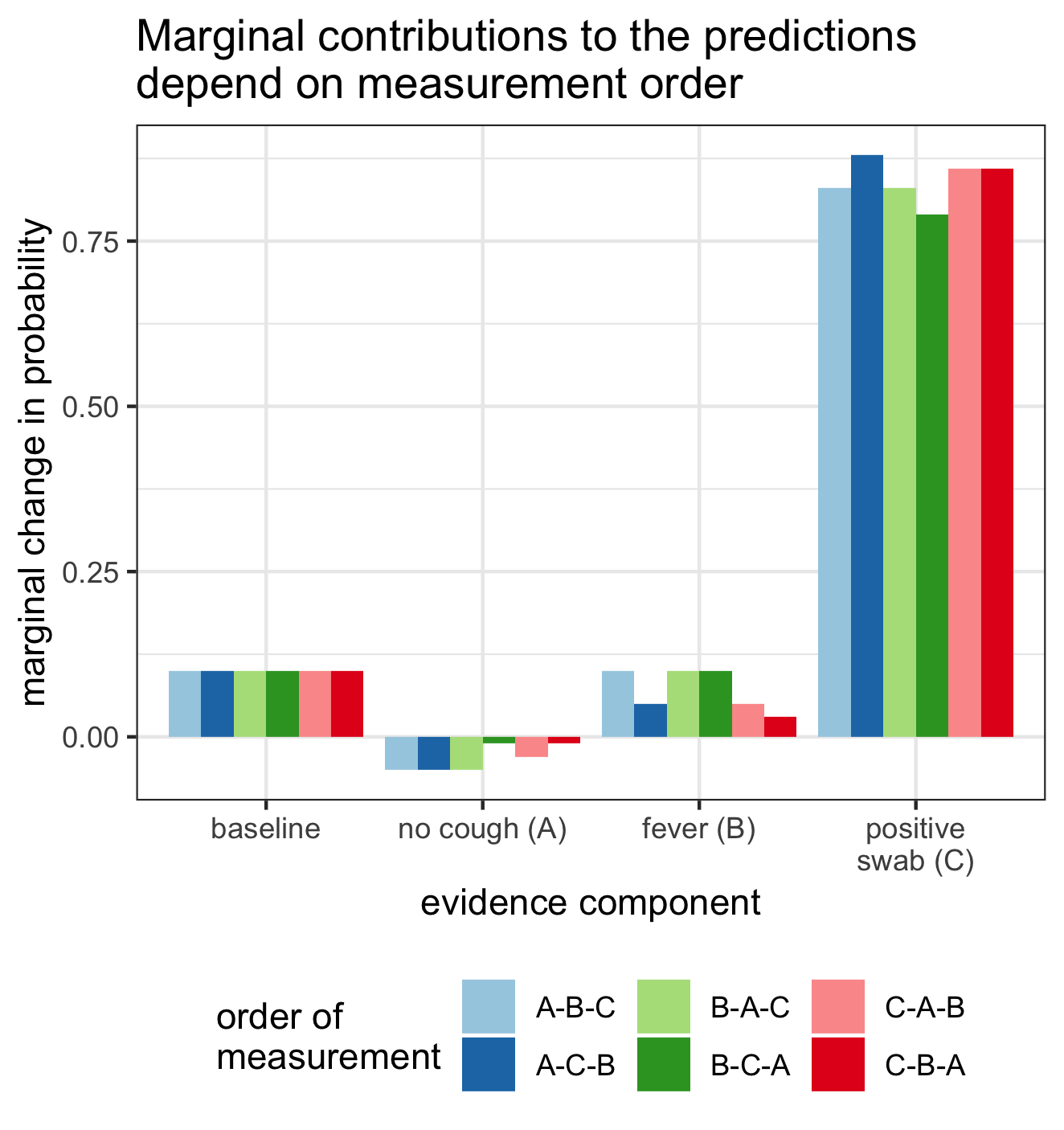
We can see from the plot above that the marginal contribution of the fever evidence is highly dependent on which measurements precede it. For example, if fever (B) is measured first, followed by the swab test (C), then the fever evidence increases our risk prediction by 0.10 (order B-C-A). Alternatively, if we first see that a health-care worker has a positive swab test (C), and then see that they have a fever (B), then the marginal contribution of the fever evidence is only 0.03. In this ordering (C-B-A), the swab test has already increased our predicted probability to almost 1, and there is little room left for the fever evidence to increase it further.

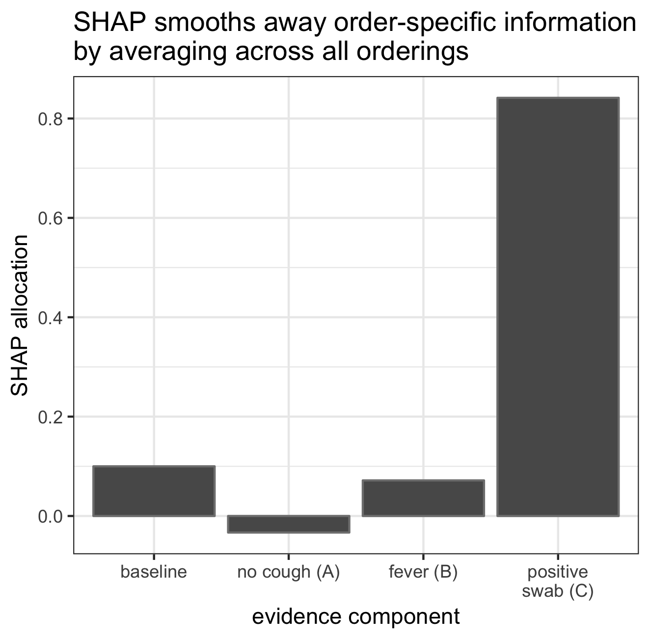
The SHAP approach defines the overall contribution of a piece of evidence as the average change in prediction induced by measuring that piece of evidence, where the average is taken across all possible orderings. These averages are shown below. By construction, the sum of the SHAP components equals the original prediction of 0.98.

L&L Theorem 1 claims that the SHAP approach is the only method that satisfies a certain set of intuitive conditions. In particular, the authors claim that this uniqueness holds even without a commonly used a "Symmetry" condition that requires the model explanation to not be influenced by external knowledge about either the problem domain or the order in which variables tend to be measured (details below).

The primary purpose of this comment is to point out that this theorem is in error. If external knowledge is allowed to influence the model explanation, then taking any weighted combination over the orderings will still satisfy the same set of intuitive conditions in Theorem 1. For example, in the COVID-19 scenario discussed here, it may be known a priori that nasal swabs are rarely collected before a fever or cough checks. Thus, analysts might wish to down-weight measurement orderings that start with a swab test. Doing so would still satisfy the Theorem 1 conditions, as written. In contrast, giving equal weight to orderings that start with a swab test could lead us to underestimate the practical value of fever and cough checks, as these checks only add substantial value when collected first.

In the next section, I'll introduce notation that will let us make this argument more specific. I'll then review L&L Theorem 1, and formally state the counterclaim that any weighted combination of feature orderings satisfies the same Theorem 1 conditions. I'll close by discussing some implications.

For context, it is important to mention that there is open debate on how transparency in machine learning should be formalized (Miller, 2017; Ray Hong et al., 2020), and on whether or not the formalization employed in SHAP has an actionable interpretation (Slack et al. (2019); Sundararajan & Najmi, 2019; Kumar et al., 2020 ). These broader questions are beyond the scope of this comment.

Notation

Here I'll introduce notation to denote input features for a model, and orderings for those features. I'll simplify away some of L&L's notation that is used to compare SHAP with other methods in the literature, and that isn't strictly needed for the L&L Theorem 1 statement. I'll also slightly modify some of L&L's notation with the goal of allowing clearer discussion. For readers interested in making a side-by-side comparison, a more detailed exposition is in Appendix 2.

Let \(\mathbf{Z}\in \mathbb{R}^m\) be an \(m\)-length random vector denoting inputs to a prediction model \(f:\mathbb{R}^m\rightarrow\mathbb{R}\), and let \(\mathbf{z}\) denote realizations of \(\mathbf{Z}\). For any vector \(\mathbf{a}\), let \(\mathbf{a}_i\) denote it's \(i^{th}\) element. Let \(\delta^{(j)}\) be an \(m\)-length vector with \(1\) in the \(j^{th}\) position and zeros elsewhere, and let \(\delta^{(0)}\) be an \(m\)-length vector of zeros. That is, \(\delta^{(j)}_i=1(i=j)\), where \(1\) is the indicator function.

Recall that in the COVID-19 example above, we considered settings where analysts had to make predictions based on only partial information. For example, when told only that a health-care worker had a fever, the analyst predicted a 20% probability of infection.

From here on, we will represent partial information by allowing \(\mathbf{Z}\) to be partially censored. Let \(\mathbf{O} \in \{0,1\}^m\) be the random variable such that \(\mathbf{O}_i=1\) if the \(i^{th}\) element of \(\mathbf{Z}\) is observed, and \(\mathbf{O}_i=0\) if it is censored. Let \(\mathbf{o}\) denote realizations of \(\mathbf{O}\). Let \((\mathbf{z}^{\text{new}},\mathbf{o}^{\text{new}})\) be a new observation of interest, where \(\mathbf{o}^{\text{new}}=\mathbf{1}_m\) is an \(m\)-length vector of ones representing no censoring, and \(\mathbf{z}^{\text{new}}\) is an input for which we want to explain the prediction \(f(\mathbf{z}^{\text{new}})\). In other words, we aim to explain a prediction, \(f(\mathbf{z}^{\text{new}})\), that was made under full information, \(\mathbf{o}^{\text{new}}=\mathbf{1}_m\).

To describe what would have happened if only partial information had been observed, let \(f_{\mathbf{z}^{\text{new}}}(\mathbf{o})\) represent the prediction that would have been made if only the subset of information \(\{ \mathbf{z}_{i}^{new} \, :\, \mathbf{o}_i=1\}\) had been available, where \(f_{\mathbf{z}^{\text{new}}}\) is a function from \(\{0,1\}^m \rightarrow \mathbb{R}\). For example, L&L choose to define \(f_{\mathbf{z}^{\text{new}}}(\mathbf{o})\) by assuming that the prediction model \(f\) includes some kind of subroutine for imputing the censored values \(\{ \mathbf{z}_{i}^{new} \, :\, \mathbf{o}_i=0\}\). It follows from this interpretation that \(f_{\mathbf{z}^{\text{new}}}(\mathbf{1}_m)=f(\mathbf{z}^{\text{new}})\). Or, in words, we know that the prediction that would have been produced from full information (\(f_{\mathbf{z}^{\text{new}}}(\mathbf{1}_m)\)) must equal the prediction that actually occurred (\(f(\mathbf{z}^{\text{new}})\)). In L&L Theorem 1, any function \(f_{\mathbf{z}^{\text{new}}}:\{0,1\}^m \rightarrow \mathbb{R}\) may be chosen so long as \(f_{\mathbf{z}^{\text{new}}}(\mathbf{1}_m)=f(\mathbf{z}^{\text{new}})\) (see Appendix 2). I'll refer to \(f_{\mathbf{z}^{\text{new}}}\) as a "partial information" function.

I'll denote the set of all \(m!\) possible input feature orderings by \(\mathcal{R}_m\). Given an ordering \(\mathbf{r} \in \mathcal{R}_m\), I'll use \(\Delta^{(\mathbf{r},i)}\) to represent the set of variables measured before \(\mathbf{z}_i\) in the ordering \(\mathbf{r}\). Specifically, let \(\Delta^{(\mathbf{r},i)}\) be the binary vector where \(\Delta^{(\mathbf{r},i)}_j=1\) if \(j\) precedes \(i\) in ordering \(\mathbf{r}\), and \(\Delta^{(\mathbf{r},i)}_j=0\) otherwise. It follows that \(\Delta^{(\mathbf{r},i)}+\delta^{(i)}\) represents the variables indices that precede \(i\) in the ordering \(\mathbf{r}\) as well as \(i\) itself. As an example to reinforce this notation, let's consider the case where \(m=3\). Here, we have

Above, the ordering \((3,1,2)\) indicates that \(z_3\) is observed first, followed by \(z_1\), followed by \(z_2\). Continuing this example, if we set \(\mathbf{r}=(3,1,2)\), then

• \(\Delta^{(\mathbf{r},1)} = (0,0,1)\) indicates that only \(z_3\) is measured before \(z_1\) in the ordering \(\mathbf{r}=(3,1,2)\);
• \(\Delta^{(\mathbf{r},2)} = (1,0,1)\) indicates that \(z_1\) and \(z_3\) are measured before \(z_2\) in the ordering \(\mathbf{r}=(3,1,2)\); and
• \(\Delta^{(\mathbf{r},3)} = (0,0,0)\) indicates that no variables are measured before \(z_3\) in the ordering \(\mathbf{r}=(3,1,2)\).

This notation will let us describe how predictions change as more and more information is acquired, in different orders.

As an aside, L&L also consider a case where \(\mathbf{o}^{\text{new}}\) can contain zeros, but it will turn out that we can simplify notation without substantively changing the Theorem 1 result if we assume \(\mathbf{o}^{\text{new}}=\mathbf{1}_m\). Similarly, L&L consider an alternate interpretation where \(\mathbf{O}\) may represent arbitrary "simplified" summaries of \(\mathbf{Z}\), but this alternative interpretation does not change the formal result in Theorem 1. Both of these topics are discussed in more detail in Appendix 2.

L&L Theorem 1 statement

Our goal is to choose a set of functions \(\{\phi_1,\dots ,\phi_m\}\) to decompose the prediction \(f(\mathbf{z}^{\text{new}})\) into components associated with each of the \(m\) features. Specifically, let \(\phi_i(f_{\mathbf{z}^{\text{new}}})\) be a real number representing the component of the prediction \(f(\mathbf{z}^{\text{new}})\) assigned to the \(i^{th}\) observed input feature, \(\mathbf{z}_i^{\text{new}}\). The value of \(\phi_j(f_{\mathbf{z}^{\text{new}}})\) may be positive or negative, with negative values roughly interpreted as saying that "in the process of measuring more and more inputs and producing increasingly refined predictions, observing that \(\mathbf{Z}_j=\mathbf{z}_j^{\text{new}}\) tends to reduce our intermediate predictions."

L&L Theorem 1 claims that, given \(f_{z^{\text{new}}}\), there is only one set of allocation functions \(\{\phi_1,\dots ,\phi_m\}\) that satisfies two specific conditions.²

L&L Theorem 1: Given a partial information function \(f_{z^{\text{new}}}:\{0,1\}^m\rightarrow \mathbb{R}\) satisfying \(f_{z^{\text{new}}}(\mathbf{1}_m)=f(\mathbf{z}^{\text{new}})\), there is only one set of functions \(\{\phi_1(f_{\mathbf{z}^{\text{new}}}),\dots ,\phi_m(f_{\mathbf{z}^{\text{new}}}) \}\) that satisfy the following 2 properties.

1. (Local Accuracy) \(f(\mathbf{z}^{\text{new}}) = f_{z^{\text{new}}}(\mathbf{0}_m) + \sum_{i=1}^m \phi_i(f_{\mathbf{z}^{\text{new}}})\), where \(\mathbf{0}_m\) is an \(m\)-length vector of zeros and \(f_{z^{\text{new}}}(\mathbf{0}_m)\) represents the baseline prediction. That is, the components \(\phi_i(f_{\mathbf{z}^{\text{new}}})\) add up to the original prediction \(f(\mathbf{z}^{\text{new}})\).
2. (Consistency) Let \(\mathbf{o}\setminus i = \mathbf{o}(1-\delta^{(i)})\) denote setting the \(i^{th}\) element of \(\mathbf{o}\) to zero. For any two models \(f\) and \(\tilde{f}\) with associated partial information functions \(f_{z^{\text{new}}}\) and \(\tilde{f}_{\mathbf{z}^{\text{new}}}\) respectively, if
   \begin{equation*} \tilde{f}_{\mathbf{z}^{\text{new}}}(\mathbf{o})-\tilde{f}_{\mathbf{z}^{\text{new}}}(\mathbf{o}\setminus i) \geq f_{z^{\text{new}}}(\mathbf{o}) - f_{z^{\text{new}}}(\mathbf{o}\setminus i) \end{equation*}
   for all \(\mathbf{o}\in\{0,1\}^m\), then \(\phi_i(\tilde{f}_{\mathbf{z}^{\text{new}}})\geq \phi_i(f_{\mathbf{z}^{\text{new}}})\). In words, this means that if the prediction strategy (\(f_{\mathbf{z}^{\text{new}}}\)) changes in such a way that the update caused by learning \(\mathbf{Z}_i=\mathbf{z}^{\text{new}}_i\) does not decrease, then the \(i^{th}\) prediction component does not decrease.

The unique set of functions that satisfies the above conditions is equal to³

In Eq (\(\ref{shap-def}\)), the term in the summation is the change in predictions caused by adding \(\mathbf{z}_i\) within the ordering \(\mathbf{r}\). In light of this result, SHAP decomposes predictions using Eq (\(\ref{shap-def}\)).

Counterclaim to L&L Theorem 1: any weights work

Eq (\(\ref{shap-def}\)) defines the component of the prediction associated with the \(i^{th}\) feature by averaging over all possible feature orderings, giving each ordering equal weight. However, the conditions in L&L can actually be satisfied by any weighting scheme for the feature orderings. This can be formalized as follows.

Counterclaim: Let \(w:\mathcal{R}_m\rightarrow \mathbb{R}\) be a weighting function satisfying \(\sum_{\mathbf{r}\in \mathcal{R}_m} w(\mathbf{r}) = 1\) and \(w(\mathbf{r})\geq 0\) for all \(\mathbf{r}\in \mathcal{R}_m\). Given any such weighting function, the decomposition functions \(\{\bar{\phi}_{1}^{(w)},\dots,\bar{\phi}_{m}^{(w)}\}\) defined as

also satisfy the Local Accuracy and Consistency conditions in L&L Theorem 1.

(Proof in Appendix 1.)

Eq (\(\ref{dist-def}\)) can also be interpreted as treating the order \(\mathbf{r}\) as a random vector following the distribution implied by \(w\), and viewing \(\bar{\phi}_{i}^{(w)}(f_{\mathbf{z}^{\text{new}}})\) as the expected change in predictions when the information \(\mathbf{Z}_i=\mathbf{z}^{\text{new}}_i\) is learned. Setting \(w(\mathbf{r})=\frac{1}{m!}\) (i.e., a uniform distribution over orderings) produces the solution in Eq (\(\ref{shap-def}\)). But, again, any weighting scheme can be used while still maintaining the conditions in Theorem 1.

Discussion

When discussing L&L Theorem 1, it's helpful to review some of the background literature that inspired SHAP. In the remainder of this comment I'll review this background and also discuss some general, open questions.

Background on SHAP, Shapley values, and the "Symmetry" condition

As the name suggests, the SHapley values for Additive exPlanations (SHAP) method is based on the Shapley value framework, a well-known concept from the game theory literature.⁴ The Shapley value framework was originally introduced in 1951 as a way to take the proceeds generated by a team and fairly distribute those proceeds to the team members. This question of how to allocate proceeds is nontrivial, especially when the total value produced by a collaborative team is different from the sum of the values that each team member would produce alone. If the cost of recruiting each individual team member can be incorporated into the net value produced by the team, then it follows that the order in which team members are recruited should not be seen as particularly important. For this reason, the Shapley value solution for distributing payments effectively ignores the order in which players are added to a team. As a result, the method uniquely satisfies three specific fairness criteria, which can be roughly described as

1. (Efficiency) the sum of payments equals the total value generated by the team;
2. (Monotonicity) if the task assigned to the team changes in such a way that the marginal contribution of the \(i^{th}\) member to any subteam does not decrease, then the payout to the \(i^{th}\) member will not decrease;⁵
3. (Symmetry) any 2 members who are equivalent, in that they make the same marginal contributions to any subteam, are payed equally.

L&L, 2017 showed that the Shapley value framework can also be applied to explain a black-box model's predictions. L&L interpret the set of input features as team members producing a prediction, and use the Shapley value framework to decompose this prediction into components associated with each of the inputs. In this context, Efficiency can be written as Local Accuracy; Monotonicity can be written as Consistency (L&L Theorem 1); and Symmetry can be written as saying that two inputs (\(i,j\)) must be assigned the same decomposition value if they make the same marginal contribution to any subset of other inputs.

That is, if \(f_{z^{\text{new}}}(\mathbf{o}+\delta_i) = f_{z^{\text{new}}}(\mathbf{o}+\delta_j)\) for all \(\mathbf{o}\in\{0,1\}^m\) such that \(\mathbf{o}_i=\mathbf{o}_j=0\), then \(\phi_i(f_{\mathbf{z}^{\text{new}}})=\phi_j(f_{\mathbf{z}^{\text{new}}})\).

It follows from the literature on the Shapley value framework that, given a partial information function \(f_{\mathbf{z}^{\text{new}}}\), the conditions of Local Accuracy, Consistency & Symmetry are sufficient to identify a unique decomposition of the prediction \(f(\mathbf{z}^{\text{new}})\). Thus, L&L Theorem 1 can be read as saying that Symmetry is not required in the context of explaining predictions, and that Efficiency and Monotonicity are sufficient to uniquely identify a way to decompose those predictions. The error in L&L Theorem 1 occurs in Line (9) of the proof (see L&L supplement). This line only follows under an implicit "Anonymity" condition that the names of input variables cannot affect the explanation. This implicit condition has previously been shown to be stronger than Symmetry (see Peters, 2008: pages 245 & 257).

It's also worth noting that the Symmetry condition has a clearer justification in the game theory setting, where the cost of recruiting a team member can be directly added to the total net value produced by the team. Again, once the cost of recruiting each team member has been accounted for, the order in which members are recruited can reasonably be described as arbitrary. In contrast, the cost of measuring a prediction model input cannot be "added" to the prediction produced by all of the inputs together, as the measurement cost and final prediction are on different scales (e.g., dollars versus probability of infection). In the context of prediction models, the measurement order often reflects the measurement costs.

In the context of the explainability literature, SHAP's attention to sequential measurement distinguishes it from many other existing methods, such as dropping a variable and retraining (see Gevrey et al., 2003), permutation-based methods (Breiman, 2001; Fisher et al., 2019), or partial dependence plots (Friedman, 2001; see also Goldstein, 2017). These alternative methods study how a model's behavior changes when only the variable of interest is altered or censored. In contrast, SHAP studies how a model's predictions change when all variables are censored sequentially (or, equivalently, when they are measured sequentially). This conceptual distinction leads to the Local Accuracy property of SHAP, a property that is not shared by the other methods mentioned above.

General discussion, and remaining open questions

We've seen that the conditions in L&L Theorem 1 are maintained even after reweighting the SHAP formula (Eq (\(\ref{shap-def}\))) using any weighting scheme, or probability distribution, over input feature orderings. This means that in order for the SHAP decomposition to be uniquely defined, a researcher must choose not only a function \(f_{z^{\text{new}}}\) to assign values to subsets of inputs (Sundararajan & Najmi, 2019), but also a weighting function \(w\) over the order in which inputs are measured.

Requiring a Symmetry condition collapses this choice to uniform weights (Eq (\(\ref{shap-def}\))), but it is not obvious that uniform weights are ideal when external knowledge is available. Frye et al. (2019) make a similar point about choosing a distribution over orderings, and argue that such a choice should reflect known causal structure. Alternatively, the order might reflect how expensive each feature is to measure (see also Lakkaraju & Rudin, 2017).

That said, there are still scenarios where equal weights can be a reasonable default choice. For example, when debugging a model it can be useful to explore a variety of explanatory methods, including SHAP (with equal weights or unequal weights), partial dependence plots, permutation importance, and more. Each method provides a new chance to understand when and why the model performs poorly.

One potential future question is whether or not all solutions to L&L Theorem 1 take the form of Eq (\(\ref{dist-def}\)). Another open question is whether there are variations of the Symmetry condition that imply different choices for \(w\). On the other hand, it might be more straightforward for a researcher to choose a partial information function \(f_{z^{\text{new}}}\) and weighting function \(w\), and then define the decomposition method as a function of \(f_{z^{\text{new}}}\) & \(w\) using Eq (\(\ref{dist-def}\)). That is, it might be easier for researchers to choose a weighting function \(w\) than to identify a variation of the Symmetry requirement that uniquely determines \(w\).

Appendix 1: Proof of counterclaim

I'll start by showing that the Theorem 1 conditions can also be satisfied by a decomposition that depends on only one feature ordering. It will follow that any weighting scheme (or distribution) over feature orderings also satisfies the Theorem 1 conditions.

A counter example from one feature ordering

Let \(\mathbf{r}\in \mathcal{R}_m\) be an arbitrary ordering of the inputs, and let

The right-hand side of Eq (\(\ref{oneR}\)) can be read as saying "within the ordering \(\mathbf{r}\), we compare the prediction made from the inputs up to and including \(\mathbf{z}_i\) against the prediction made based only on the inputs measured strictly before \(\mathbf{z}_i\)."

For Property 1 (Local Accuracy), we see that

Above, Line (\(\ref{reorder}\)) comes from reordering the summation terms. Line (\(\ref{zeroM}\)) comes from the fact that \(\Delta^{(\mathbf{r},\mathbf{r}_1)}=\mathbf{0}_m\), as no variables occur before \(\mathbf{r}_1\) in the ordering \(\mathbf{r}\). Line \((\ref{backup})\) comes from the fact that \(\Delta^{(\mathbf{r},\mathbf{r}_i)}=\Delta^{(\mathbf{r},\mathbf{r}_{i-1})}+\delta^{(\mathbf{r}_{i-1})}\) for \(1< i\leq m\), that is, the integers preceding the \(\mathbf{r}_i\) in order \(\mathbf{r}\) are equal to the integers preceding \(\mathbf{r}_{i-1}\) as well as \(\mathbf{r}_{i-1}\) itself.

For Property 2 (Consistency), suppose we know that

for all \(\mathbf{o}\in\{0,1\}^m\). We can apply the above relation at \(\mathbf{o}=\Delta^{(\mathbf{r},i)}+\delta^{(i)}\) to get

Thus, \(\bar{\phi}_{\mathbf{r},i}(f_{\mathbf{z}^{\text{new}}})\) satisfies the conditions in L&L Theorem 1, but is not equal to \(\phi_{i}(f_{\mathbf{z}^{\text{new}}})\) (see Eq (\(\ref{shap-def}\))), and so these conditions are not sufficient to identify a unique set of decomposition functions. Note however that \(\bar{\phi}_{\mathbf{r},i}(f_{\mathbf{z}^{\text{new}}})\) does not satisfy the Symmetry condition (see background section, above), and so would not contradict Theorem 1 if a Symmetry condition was added to Theorem 1.

Generalizing the counter example to weight all possible orderings

Building on the previous section, we'll now treat the weighting scheme \(w\) as a discrete probability distribution over all possible orderings. That is, we'll say that \(P(\mathbf{R}=\mathbf{r})=w(\mathbf{r})\), where \(\mathbf{R}\in \mathcal{R}_m\) is a random ordering. This means that, given \(w\), the function \(\bar{\phi}_{i}^{(w)}(f_{\mathbf{z}^{\text{new}}})\) is the expected value of \(\bar{\phi}_{\mathbf{R},i}(f_{\mathbf{z}^{\text{new}}})\) (see Eq (\(\ref{oneR}\))) with \(\mathbf{R}\) following the distribution implied by \(w\).

It now follows from linearity of expectations that \(\bar{\phi}_{i}^{(w)}(f_{\mathbf{z}^{\text{new}}})\) satisfies Local Accuracy. Similarly, it follows from monotonicity of expectations that \(\bar{\phi}_{i}^{(w)}(f_{\mathbf{z}^{\text{new}}})\) satisfies Consistency. Thus, \(\bar{\phi}_{i}^{(w)}(f_{\mathbf{z}^{\text{new}}})\) satisfies the conditions in L&L Theorem 1.

Appendix 2: More detailed notes on notation

Much of the notation from L&L is used to connect SHAP with other methods in the literature, and isn't strictly needed for the topics discussed here. For readers looking at this comment side-by-side with L&L, this section lists the notation simplifications and changes I've made throughout this comment.

First, the change that is perhaps most immediately noticeable is that L&L use the notation \(z\) to denote the random inputs to \(f\), and use \(x\) to denote the realization of \(z\) for which we would like to explain the prediction. That is, L&L aim to explain the prediction \(f(x)\). I've replaced \(z\) and \(x\) with \(\mathbf{Z}\) and \(\mathbf{z}^{\text{new}}\) respectively, based on the style of upper case letters for random variables and lower case letters for realizations of those random variables.

Second, I've used the notation \(\phi_i(f_{\mathbf{z}^{\text{new}}})\) to refer to what L&L write as \(\phi_i(f,x)\). L&L's notation implicitly assumes a fixed mapping from \(f\) and \(x\) to \(f_x\). However, many such mappings could be justified, and L&L end up considering more than one (see L&L page 5). My notation here is motivated by the fact that the functions \(\phi_i\) do not depend on \(f\) except through \(f_{\mathbf{z}^{\text{new}}}\). This fact is especially relevant to the "Consistency" condition.

L&L also often abbreviate the value \(\phi_i(f,x)\) as simply \(\phi_i\), and abbreviate the full set of functions \(\{\phi_1,\dots ,\phi_m \}\) by nesting them within a function denoted by \(g\). I've omitted these abbreviations in order to distinguish functions from the values they produce.

Third, L&L let \(\mathbf{Z}\) itself contain missing values, whereas I've represented missingess with a separate variable \(\mathbf{O}\). Specifically, L&L say that the random variable \(z\) can contain missing elements, and use the notation \(z'\) to flag these missing values. Here, the apostrophe in \(z'\) is meant to represent a summary function applied to \(z\). Specifically, it represents a function that returns an \(m\)-length vector of nonmissingness indicators, such that \(z'_i=0\) when \(z_i\) is missing and \(z'_i=1\) otherwise (here, the order of operations is \(z_i'=(z')_i\)). For example, if \(z=(3,\text{NA},4.1)\) then \(z'=(3,\text{NA},4.1)'=(1,0,1)\), where here I've used \(\text{NA}\) to redundantly represents a missing value. L&L also consider a more general case where the apostrophe could represent any binary summary function applied to the random inputs \(z\), so long as there exists a reverse mapping \(h_{x}\) satisfying \(h_x(z')=z\) when \(z=x\). Note that the value of \(h_x(z')\) is unconstrained when \(z \neq x\). That said, the core theorem statement is technically not affected by how \(z'\) is interpreted. As an aside, the Local Accuracy & Missingness properties of L&L Theorem 1 become arguably less intuitive if \(x'_i\) is interpreted as something other than a nonmissingness indicator.

On a related note, I've also generally omitted the notation \(h_x\) from this comment. In the context of L&L Theorem 1, the mapping \(h_x\) is used only as way to introduce \(f_x\) (equivalently, \(f_{z^{\text{new}}}\)) by defining it as \(f_x(z')=f(h_x(z'))\). This definition comes from L&L Property 3 and L&L Eq (5), although not all of the described choices for \(f_x\) strictly satisfy this definition (see the relation that \(f_x(z')=E(f(z)|z_S)\) at the top of L&L page 5). Since \(h_x\) does not appear elsewhere in the theorem, we can omit this notation if we translate the constraints on \(h_x\) into constraints on \(f_x\). Specifically, if \(f\) can produce any number on the real line and \(h_x\) is unconstrained except for the requirement that \(h_x(x')=x\), then \(f_x\) is unconstrained except for the requirement that \(f_x(x')=f(h_x(x'))=f(x)\). Equivalently, \(f_{z^{\text{new}}}\) is unconstrained except for the requirement that \(f_{z^{\text{new}}}(\mathbf{o}^{\text{new}})=f(\mathbf{z}^{\text{new}})\). Without the assumption that \(f\) can produce any value on the real line, we have to additionally restrict \(f_{z^{\text{new}}}\) to only produce values in the range of \(f\), but this doesn't change the Theorem 1 result since \(f_{z^{\text{new}}}\) is generally viewed as given, or fixed.

Fourth, my above choice to set \(\mathbf{o}^{\text{new}}=\mathbf{1}_m\) deviates from L&L, who allow \(z'\) to contain zeros. (Recall that my notation \(\mathbf{o}^{\text{new}}\) is the analogue of \(z'\).) Accordingly, I've also omitted L&L's "Missingness Property" from Theorem 1. Implicit in L&L's assumption that \(z'\) can contain zeros is the assumption that \(f\) can handle missing values. However, the Missingness Property in L&L Theorem 1 requires that no part of the decomposition of \(f(x)\) be assigned to summary features \(x_i'\) for which \(x_i'=0\). Thus, the zero-values in \(z'\) (and hence \(\mathbf{o}^{\text{new}}\)) are effectively ignored in L&L Theorem 1. For this reason, we can adapt the above counterclaim to the case where \(\mathbf{o}^{\text{new}}\) contains zeros by fixing the zero values of \(\mathbf{o}^{\text{new}}\) and letting only the nonzero values vary. Let \(p=\sum_{i=1}^m\mathbf{o}^{\text{new}}_i\), and let \(d=m-p\) be the number of zeros in \(\mathbf{o}^{\text{new}}\). Without loss of generality, let us first assume that all zero entries occupy the last \(d\) elements of \(\mathbf{o}^{\text{new}}\). Let \(\mathbf{Z}_{\text{subset}}\in\mathbb{R}^p\) represent the first \(p\) (observed) inputs, and let \(f_{\text{subset}}(\mathbf{Z}_{\text{subset}})=f((\mathbf{Z}_{\text{subset}}, \text{NA},\dots,\text{NA}))\) be the version of our prediction function \(f\) that depends only on \(\mathbf{Z}_{\text{subset}}\). In this setting, replacing \(f\) with \(f_{\text{subset}}\) and replacing \(\mathbf{Z}\) with \(\mathbf{Z}_{\text{subset}}\) produces an equivalent problem of explaining the prediction \(f_{\text{subset}}((\mathbf{z}^{\text{new}}_1,\dots,\mathbf{z}^{\text{new}}_p))=f(\mathbf{z}^{\text{new}})\), but with inputs \((\mathbf{z}^{\text{new}}_1,\dots,\mathbf{z}^{\text{new}}_p)\) that are fully uncensored.

Finally, readers might note that Eq (\(\ref{shap-def}\)), above, is different from that of L&L Eq (8). We can relate these two equations by noting that

where the term in curly braces is the number of orderings in which the indices \(\{j\,:\,\mathbf{o}_j=1\}\) occur first, followed by \(i\), followed by the remaining indices \(\{j\neq i\,:\,\mathbf{o}_j=0\}\). The remaining difference between the two formulas is due to a small typo in L&L Eq (8), as noted in the authors' Errata document.

Acknowledgments

Thanks very much to Scott Lundberg, Beau Coker & Berk Ustun for their invaluable help in process of writing this comment.